micrograd: six gradient rules and a loss floor I should have predicted

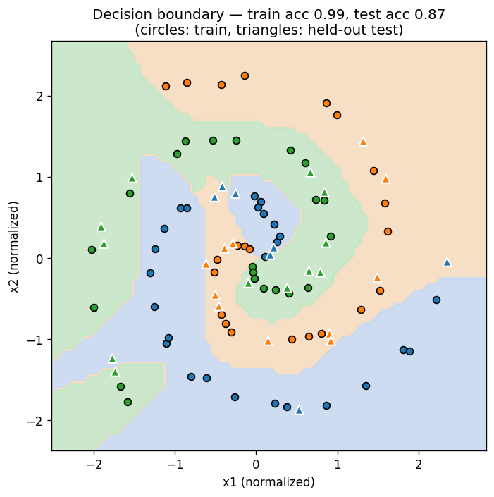
I rebuilt micrograd — Karpathy’s scalar autograd engine — from scratch, following his Zero to Hero lecture: a Value class that builds a computation graph through Python operator overloading, then runs reverse-mode automatic differentiation over it. Scalar-valued means every neuron gets decomposed into its individual adds and multiplies — hopeless for performance, ideal for seeing the mechanism, since each node in the graph carries exactly one number and one gradient. On top of the engine sits a small neural net library (Neuron, Layer, MLP), a test suite that checks every gradient against PyTorch, and a demo that trains an MLP on three interleaved spirals — a 2D, three-class problem I generate directly, without sklearn. The packaging, the gradient tests, and the spiral experiment are mine. Code: github.com/diego-magana/micrograd.

The reason I did this is that I didn’t want backpropagation to be something I trust loss.backward() to do. Karpathy’s argument for why you shouldn’t is that backprop is a leaky abstraction — stack layers, trust the framework, and the failure modes find you anyway, just later and with worse debugging information. Building the engine is taking that argument literally: I wanted to have written the actual lines where gradients get computed. It turns out there are only six of them — and the most instructive things I hit along the way had nothing to do with the calculus.

The whole engine is six gradient rules

Three operator rules:

\[\frac{\partial}{\partial a}(a+b) = 1 \qquad \frac{\partial}{\partial a}(ab) = b \qquad \frac{\partial}{\partial a}(a^n) = na^{n-1}\]

and three elementary functions: $\tanh$ (derivative $1 - \tanh^2 x$), $e^x$ (its own derivative), $\ln x$ (derivative $1/x$). Each rule is a closure registered on the output node at the moment the operation runs — multiplication, for instance:

def __mul__(self, other):
    out = Value(self.data * other.data, (self, other), '*')
    def _backward():
        self.grad  += other.data * out.grad   # d(ab)/da = b
        other.grad += self.data  * out.grad   # d(ab)/db = a
    out._backward = _backward
    return out

Each gradient rule is one line of chain rule: local derivative times whatever gradient arrived from above.

The forward pass builds the graph as a byproduct of Python’s operator dispatch. The backward pass is nothing but these closures fired in the right order. Everything else on the public surface — subtraction, division, negation, the reflected __r*__ variants — composes from the primitives: subtraction is addition of a negation, division is multiplication by a power of −1. None of them defines a backward rule, and none needs to. (Six rules cover everything in this post; the engine registers two more. sigmoid is a convenience the six can already express as $1/(1+e^{-x})$, implemented directly so large negative inputs don’t overflow exp. relu is not — it needs a comparison rather than an arithmetic operation, so it genuinely extends what the engine can express. Neither shows up anywhere in this post.)

The part that made this click for me: I built softmax and negative log-likelihood loss purely out of exp, log, addition, and division over Value objects, and the engine produced the textbook gradient

\[\frac{\partial L}{\partial z_i} = p_i - \mathbb{1}[i = y]\]

on its own. That result — probability minus one for the correct class, probability for the rest — is usually derived on a whiteboard with careful bookkeeping. Here it falls out of the chain rule applied mechanically over the graph. And it reads like an instruction: pull the correct class up by exactly the probability it’s still missing, push every other class down by exactly the probability it grabbed. Nothing in the engine knows what softmax is, and it matches PyTorch to 1e-5.

This composition is also the hardest test the engine faces, because the softmax denominator creates a diamond: $e^{z_i}$ feeds its own numerator and the shared $\sum_j e^{z_j}$, so during the backward pass its gradient arrives along two paths that have to be summed. If gradient accumulation is broken anywhere, this is where it shows.

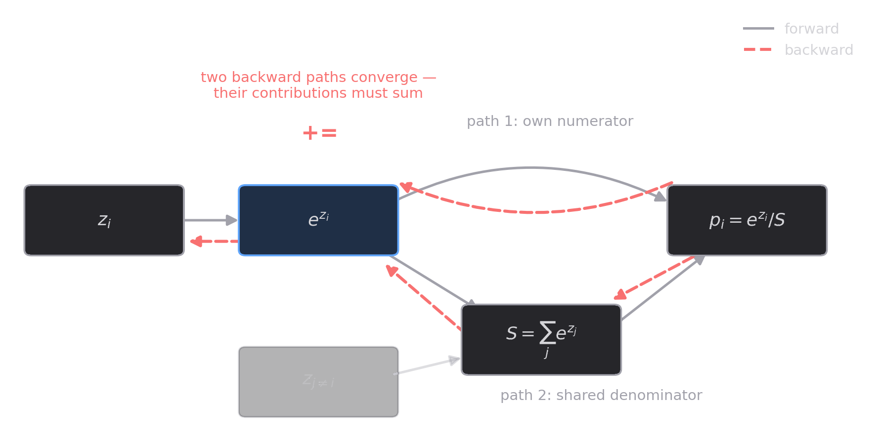The softmax diamond. $e^{z_i}$ has two consumers — its own numerator and the shared denominator — so two backward paths (red) converge on it and their contributions must sum. This one structure exercises every primitive in the engine plus the accumulation rule.

That’s the real economy of the design: derived operations don’t need derived gradients. Six local rules plus the chain rule differentiate any composition built from them — including compositions the engine has never heard of.

The bugs that matter don’t crash

The unpleasant thing about writing an autograd engine is that its worst bugs are silent. Wrong gradients don’t throw exceptions. Loss often still decreases. You get a network that trains — on the wrong numbers.

Two of these are structural. The backward closures have to accumulate with +=, never assign with =: y = x * x reuses x, and $dy/dx = 2x$ only because two contributions sum at the node. Assign instead and the second path silently overwrites the first — at $x = 3$ you get a gradient of 3 instead of 6. Wrong exactly when a value is reused, which in a real network is everywhere. And backward() has to walk the graph in reverse topological order: each closure distributes out.grad to its operands, so out.grad must already hold every downstream contribution before the closure fires. This is the same dependency problem a compiler solves when it schedules expression evaluation. Skip the sort and some nodes propagate partial gradients. No error — just wrong.

The third is easy to miss because it hides in an ordinary line of Python — and in this engine it hides inside the softmax itself. Building the denominator is sum(counts), and sum() starts from the integer 0, so the first operation is 0 + Value — int.__add__ fails, and Python falls back to Value.__radd__. Without the reflected operators, the engine works in every expression I write by hand and breaks the first time a standard-library idiom touches it. I stopped thinking of __radd__ and friends as polish; they’re what makes the type behave like a number.

Since none of this announces itself, the tests are the correctness argument, not hygiene. I verified every operator — and the full softmax+NLL composition, diamond included — against PyTorch’s autograd. The assertion is 1e-5 absolute, which on the tangled test case works out much tighter than it sounds: the gradients there reach $10^5$, so that’s agreement to eleven significant figures. Two independent implementations matching that closely means the graph construction and the chain-rule application are both right. One detail: I cast the PyTorch reference tensors to float64, because the default float32 floors the comparison around 1e-7 and fails tests against Python floats for no real reason.

The claim that these bugs are silent is itself testable, so the suite tests it. test_accumulation_is_not_assignment swaps the += for =, trains a small MLP on thirty points, and asserts the loss still falls — 46.3 down to under 12, on a network where every gradient is wrong.

It’s worse than silent. Run the broken version twice and you get different answers — 8.77, 9.55, 11.42 from identical seeds — because backward() orders the graph by iterating a set of nodes hashed by identity, so traversal order shifts with memory layout between runs. With += that’s invisible: every path contributes and addition commutes. With = the last writer wins, and which node writes last is an accident. Which means the second bug here isn’t independent of the first — accumulation is what makes the traversal order stop mattering.

A loss floor I should have predicted

My first demo trained MLP(2, [16, 16, 1]) — 337 parameters — on make_moons(n=100, noise=0.1): 100 epochs of full-batch SGD at learning rate 0.01, binary cross-entropy on a sigmoid of the output.

Accuracy reached 100/100 and the decision boundary separated both classes cleanly. But the summed loss plateaued at 31.84 and would not move. My first instinct was a bug — stale gradients, a broken update step, something in the engine.

It’s arithmetic. The output neuron is tanh-activated, so the value going into the sigmoid lives in $(-1, 1)$, and the predicted probability is capped:

\[p = \sigma(z) < \sigma(1) \approx 0.731\]

The best possible per-sample BCE is $-\ln(0.731) \approx 0.313$, so over 100 samples the minimum achievable loss is about 31.33. The network sits at 31.84 — within ~1.6% of a floor its own architecture imposes. It classifies everything correctly and is structurally forbidden from being confident about any of it.

scripts/loss_floor.py in the repo rebuilds that network so this is checkable rather than remembered. It has to stack the layers by hand, because MLP won’t produce a tanh head any more — that’s the fix, below. A fresh run lands at 32.20 against the same 31.33: the floor reproduces, the exact historical number doesn’t.

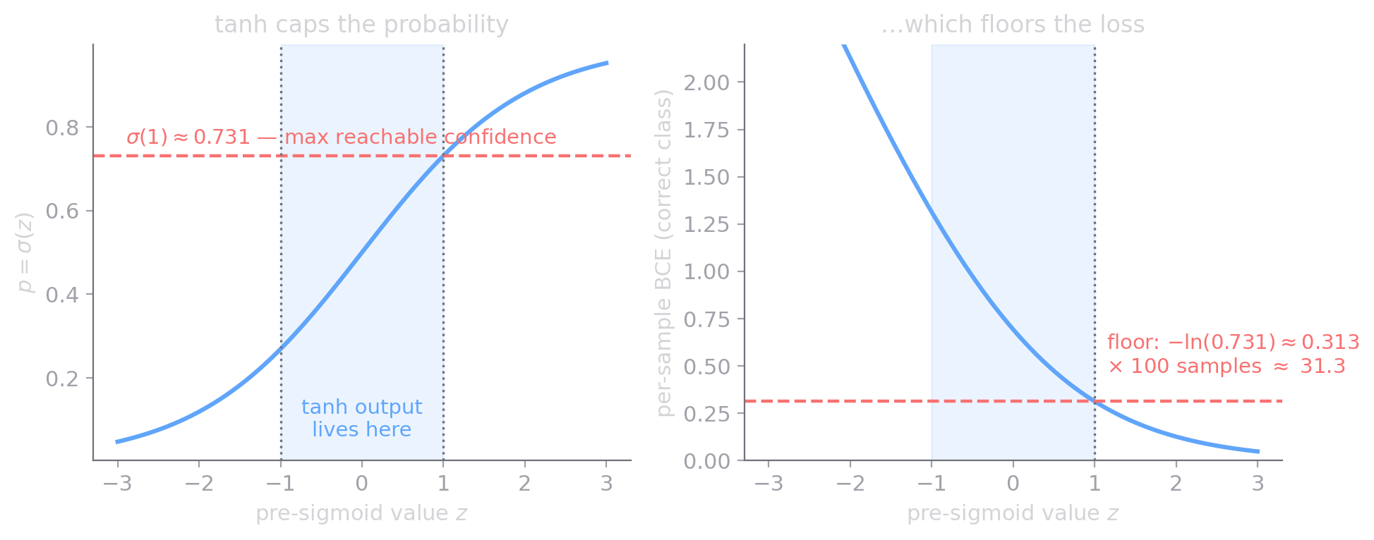The whole “bug” in two panels. Left: the tanh output confines the pre-sigmoid value to the shaded band, capping confidence at $\sigma(1) \approx 0.731$. Right: that cap floors the per-sample loss at 0.313 — times 100 samples, the 31.3 that explains the 31.84 on my screen.

What I didn’t expect is that the same property of tanh shows up at both ends of the network with opposite consequences. At the input, saturation is a gradient problem — large inputs push activations toward ±1, where $1 - \tanh^2 x \to 0$ and learning stalls, which is why I normalize the features to zero mean and unit variance before training. At the output, saturation is a confidence problem — the same boundedness that makes tanh a well-behaved hidden activation makes it the wrong thing to put in front of a sigmoid. One function, two failure surfaces, and only one of them shows up in the gradients.

Except they aren’t two events. Invert the number: a summed loss of 31.84 over 100 samples is a mean BCE of 0.3184, so the mean predicted probability is $e^{-0.3184} = 0.727$, which puts the tanh output at 0.981 — and there the local gradient $1 - \tanh^2$ is 0.0376. The output neuron was pinned against its ceiling and passing back four percent of the gradient it received. The confidence cap and the vanishing gradient are the same saturation, read from two ends.

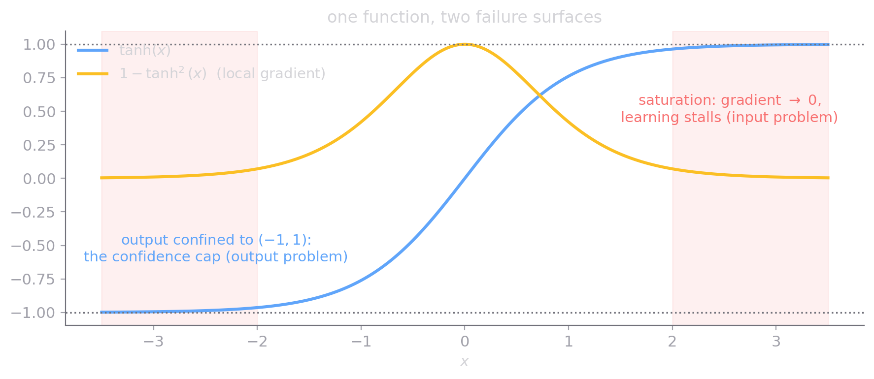tanh’s two failure surfaces. In the shaded zones the local gradient (gold) vanishes and learning stalls — the input-side problem. The output range never leaves $(-1, 1)$ — the output-side problem that produced the loss floor.

The habit I’m keeping from this: I could have computed the floor before training, from the architecture alone. When a loss curve plateaus, the first question isn’t which learning-rate schedule to try — it’s what the minimum achievable loss actually is under the model’s output parameterization. Sometimes the plateau is the answer.

The fix is the one every framework quietly uses: a linear output layer that emits unbounded logits and leaves the squashing to the loss function. The current demo in the repo applies it directly — MLP(2, [16, 16, 3]), 371 parameters, softmax+NLL on three-class spirals with a linear output head and a real train/test split (train 0.99 / test 0.87).

The spirals are a harder problem than the moons, and I wanted that measured rather than asserted, so I ran a linear baseline: the same softmax head with no hidden layers, nine parameters. It converges to a held-out NLL of 1.14 on this split, against the $\ln 3 \approx 1.10$ of guessing uniformly. It isn’t undertrained — the training loss stops moving at step 80 and hasn’t moved by step 3,000, settling at finite weights instead of running them off toward infinity the way a linear model does when the classes really are separable. It fits the training set a little (1.00) and none of that transfers.

Accuracy says the same thing less stably: 0.27 on 30 test points, with predictions falling [14, 8, 8] against true counts of 7/11/12 — it collapses onto one class rather than separating the arms. That’s what a linear boundary does when the classes wrap around each other. It can’t draw the curve, so it picks a half-plane and eats the loss. The MLP reaches 0.87 on that same split, and the hidden layers are the entire difference.

Where this stops

The scalar design is a deliberate ceiling, not an oversight. One Value per number and a Python loop per forward pass make this $O(\text{samples} \times \text{params})$ with no vectorization — fine for a hundred 2D points, hopeless for anything real. The point was never speed. It was that you can read every gradient.

Two other boundaries worth naming. The test-below-train gap is small-data reality — a few dozen points per class with genuine overlap near the origin — rather than a bug I haven’t found. And the softmax here is the plain form: at larger logit magnitudes it needs the log-sum-exp trick to stay numerically stable, which is the first thing makemore has to fix.

What’s next

The finished engine differentiates anything I can express as a composition of its scalar operations — softmax, NLL, BCE, and an arbitrary MLP are all just graphs it walks the same way. Backpropagation stopped being a black box for me at the point where I had written all eight closures and watched an independent implementation confirm every one of them.

Next is makemore: the same foundation carried into sequence modeling, where the question shifts from whether the gradient is correct to what the network actually learned. From there it’s gpt, where answering that question properly takes ablation and activation patching rather than just reading off measurements.